Kelly for the cowardly

Kelly staking is - as we've seen before - the mathematically optimal way to grow your bankroll. It has one glaring problem, though: it's horrifically volatile. Let's imagine we make 100 bets which we know are 50-50 shots but the bookies insist on pricing at 2.10. Our Kelly stake is (po-1)/(o-1) = 4.55%.

Now, when we win, we tend to win big - about a quarter of the time, we'd get 53 or more correct. That would net us at least a 49% profit. The flip-side of that is, a quarter of the time we get 46 or fewer and lose a quarter of our bankroll. There's a one in twenty chance that we'll lose half of our bankroll (although one in ten that we'll double it). With bigger edges or shorter odds, the fluctuations can be terrifying.

Is there a way to reduce them? Well, obviously, if you don't bet so much, your bankroll is steadier. But let's say you're still pretty greedy, and want to maximise your worst plausible outcome.

How do you even define that? Well, given that we're looking at a binomial distribution, we can use stats to help us. If we look at N identical bets with probability p, we know that 97.7% of the time* we'll win at least W_min = Np - 2 sqrt(Np(1-p)) of them. Bumping up the 2 to 3 gives us 99.87% confidence.

Whatever value we choose - I'm happy enough with two - outlines our worst plausible set of results over N trials**. We can then calculate our worst plausible outcome, which is B₀ (1 + k(o-1))^Wmin(1 - k)^(N-Wmin).

The trick now is to maximise this with respect to each k. It turns out, if we define p* as Wmin/N, that our optimal Kelly stake in this sense is (p*o-1)/(o-1). And if it's less than zero, we don't bet.

This is quite restrictive - in the case above, with N = 100 we simply wouldn't bet - p* is 40%, far too low to allow us to meet our minimum. N = 1000 isn't that much better - p* = 46.8%, where we need 47.6%. N = 2500 is just about enough.

Here are the results of running 2500 bets 1000 times over (using the two staking patterns on the same events):

           Pure Kelly     Modified
Stake        4.55%           0.73%
AROI***     26.07%           3.81%
SD          64.52%          23.58%
Worst      -79.85%         -11.44%

So, on average, Kelly outperforms the modified version by some way - but at the cost of much higher risk. The modified stakes 'guarantee' that the lowest plausible value is as large as possible.

It is possible to make up the discrepancy to a fair degree by increasing N, because the larger N is, the closer p* is to p (the square root term ends up getting very small).

Modified Kelly staking is worthwhile for bets with sufficiently large edges, or over sufficiently long runs. If you plan to make only 100 bets, you would need odds of at least 2.5 on a 50-50 shot before the modified stakes allowed you to bet.

I just typed bed, which is probably a Freudian slip. It's getting late.

* Look it up in a normal distribution table.

** We needn't assume the bets are identical. In general, we can replace Np with sum(p) and the bit inside the square root would be sum( p(1-p) ). But that complicates things a bit more than we need for the proof of concept.

*** Average Return on Investment

Optimal staking subject to constraints

This came from a post in Punter's Paradise by The Dark Arts.

It's Sunday night, you've got 5 value calls on that night's NFL games. Let's say you can get 10/11 (1.909) but you make them 55% chances. However, they are each simultaneous kick off times.

What's your stake?

(BTW,I don't know the answer).

tda.

The maths for this is a mess, using partial derivatives and Lagrangian multipliers, but the stake sizes that maximise your bankroll long-term can be calculated.

Here's the situation: you make n simultaneous bets of k_i of your bankroll B₀ at o_i, each of which has probability p_i of occurring (for i = 1..n). The expected return E_i for each bet is

E_i = B₀ (1 + k_i (o_i -1)^(p_i) (1-k_i)^(1-p_i). (1)

Your expected bankroll B after the results come in is

B(k) = sum(i=1..n) E_i. (2)

However, you're subject to the constraint that you can't bet more than your entire bankroll:

g(k) := sum(i=1..n) k_i <= 1. (3)

This is a problem for Lagrangian multipliers. We want to maximise B (Eq 2) subject to the constraint (Eq 3). We then want to solve for:

∂B/∂k_i + λ ∂g/∂k_i (4), for all i, and
g(k) <= 1 (5)

The derivation is a mess, with
∂B/∂k_i = B₀ (1 + k_i (o_i-1))^(p_i-1) (1-k_i)^(-p_i) (p_io_i-1 - k_i(o_i-1)). (6)

I doubt there's a closed-form solution for this, but trial and error works - let's try a complicated case first, with two great-looking bets:

Bet .p. .o.. .k..
.1. 0.9 1.50 0.70
.2. 0.8 2.50 0.67


Our Kelly stakes add to 1.37 bankrolls and we only have one! So what's the best solution? Obviously, if we can't get as much on as we want, we should bet as much as we can, so we have a strict constraint - the <= is an equals sign. The derivatives of g are all one, so we're left with λ = ∂B/∂k_i for all i - meaning that all the derivatives of B are the same. In this case, the only solution is for λ ~ 0.225, giving stakes of 41.8% and 58.2%.

The upshot of all this is that the optimal staking strategy is when the partial derivatives ∂B/∂k_i are equal and the k_is sum to at most one. There are two scenarios: first, if the Kelly stakes generated the usual way sum to less than 1, they're optimal. This is the case in TDA's question, which I'll get back to in a minute. If not, you're going to need to get your Excel solver working hard to satisfy the constraints. Or write some code.

In TDA's question, we had p=0.55, o=1.919 and n = 5. The optimal stake on each is 0.055, making a total stake of 0.275.

The Reverend Bayes and tennis probability, Part II

For our Big Bayesian Experiment, let's take an example from 2005, which is the tennis-data spreadsheet I currently have open. Roger Federer* took on Andre Agassi in the semi-final of the Dubai Duty Free men's tournament on Feb. 26th. A little over a month earlier, they played in the quarter-finals of the Australian Open, which Federer won handily, 6-3, 6-4, 6-4.

I'm going to take a very simple model of tennis, one which could almost certainly be improved by taking into account strength of serve and the number of service breaks in each set - unfortunately, I have neither the data, the programming skill nor the patience to put that kind of model into effect for a short blog article. Anyway, contrary to all good sense, I'll assume that each game has an identical probability of each player winning, and that parameter carries forward to the next match.

And to begin with, let's also assume that we know nothing about Federer and Agassi - the chance of Federer being a Scottish no-hoper and having no chance of getting near Agassi (p_F=0, p_A=1) is the same as that of the roles being reversed (p_F=1, p_A=0) - all values of p_F are equally likely. This is our prior distribution. We're looking for a posterior distribution of p_F - how likely each value of the variable is.

There's some number-crunching to be done here. What we're going to do is examine every (well, almost) possible value of p_F, find the probability for each of Federer winning the match with that score, and examine the distribution that comes out. Some examples:


.pF. P(6-3) P(6-4) P(6-3, 6-4, 6-4)
0.40 0.0493 0.0666 0.00022
0.50 0.1091 0.1228 0.00165
0.60 0.1670 0.1505 0.00378
0.70 0.1780 0.1204 0.00258


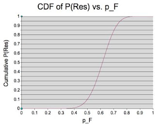
The highest of these is 0.60 (in fact, the most likely value for p_F is the number of games he won - 18 - over the number played - 29 - or about 0.62). The number-crunching (combined with NeoOffice) give a nice graph of the likelihoods, which I reproduce here:




You can see that the peak of the PDF (I won't go into the terminology here, it's getting long) is indeed around 0.62 (0.6207, to be precise). But we're interested in a confidence range, for which we read off of the CDF the p_F values for P at various levels. For instance, we're 95% certain that p_F lies between the 0.025 level and the 0.975 level - i.e. between 0.4385 and 0.7734. We're 50% sure that it lies between the 0.25 and 0.75 levels - so between 0.5550 and 0.6734.

How does this help us? Well, it narrows down p_F substantially - remember, we didn't have a clue what it was before. Now we can say with some certainty where it isn't - it's unlikely to be more than 0.7734 or less than 0.4385, eliminating almost two-thirds of the possible values at a stroke. It's as likely as not to be in the range [0.5550, 0.6734]. Can we translate this into a match probability for the next game? Of course. Again, it's a number-crunching exercise, but we get the following for our key values of p_F:


..pF.. P(Set) P(2-0) P(2-1) P(Win)
0.4385 0.3307 0.1093 0.1464 0.2557
0.5550 0.6522 0.4253 0.2959 0.7217
0.6207 0.8075 0.6250 0.2510 0.8760
0.6734 0.8977 0.8058 0.1649 0.9707
0.7734 0.9825 0.9653 0.0338 0.9991


This tells us: the most likely probability of Federer beating Agassi in two sets is 87.6% (1.14), that it's as likely as not to be between 72.17% (1.39) and 97.07% (1.03), and 95% certain to be between 25.57 (3.91) and 0.9991 (1.001). In the event, the best available odds were 1.35 with Expekt - and depending on how much confidence-in-value we wanted, we would take those and reap the benefit of Federer's 6-3, 6-1 demolition job.

This system is, I have to stress, very basic and currently only works if the two players met in the recent past. In the next instalment, I might have a shot at a link function so we can rate players who haven't met recently - but have played a common opponent.

* easy to spell; difficult to stop spelling

The Reverend Bayes and tennis probability

The Reverend Thomas Bayes was pretty much your archetypal dour, 18th century English Nonconformist minister. Except that he was a probability whizz, and gave us a law which has annoyed amateur statisticians for the better part of three centuries. It goes something like this: the probability of one thing happening given that another happens, is the probability of both happening divided by the probability of the other thing: P(A|B) = P(A & B)/P(B)

A typical example would be "Given that my girlfriend has two cats, at least one of which is female, what is the probability of her having two girl cats?" The probability of two cats both being female is (in our idealised world) one in four, or 25%. The probability of at least one female cat in two is 3/4 or 75% (FF, FM, MF all include a girl, MM doesn't). So the probability of a second girl given a first girl is (25%)/(75%) or 1/3 (33.33%) - higher than the 1/4 given no information.

It is natural that Bayes's Law should remind me of tennis, since I have spent a lot of time looking at both twisting my head from one side to the other. How can we use previous results to determine unknown probabilities? And how well do we know them?

We will need to broach the difficult subject of probability distributions. The easiest way (for me at least) to visualise a probability distribution is as a graph. The graph outlines a region of unit area* - the x axis is an outcome, often a continuum from 0 to 1 but not forcibly; the y axis is a mystical variable called probability density. You drop a pin onto the graph so that the point is equally likely to land anywhere in the region, and read off the value on the x-axis. You can see that the peaks in the graph correspond to more likely outcomes.



Let's look first at the PDF of the sum of three rolled dice. It peaks in the middle, around 10 and 11 - meaning that you're much more likely to roll 11 than 3. This makes sense - you have many more ways to roll 11 (27, I think) than to roll 3 (just one).

Some important distributions include the uniform distribution, which is a level straight line (all outcomes equally likely) and the normal distribution, which is a bell curve - outcomes near the mean are much likelier than ones far away.

What we're going to try in the next article is create a very simple tennis model and find how our knowledge about one game affects our knowledge of the next. Our strategy is going to be as follows.

We start with a uniform prior distribution of p, a variable that describes how likely one of the players is to win a single game. We then take each possible value of p (from 0 to 1) and see what the probability of the result of a known game would be, given that value of p. Out of that we get a likelihood graph showing what values of p are more likely than others - which can be converted into a PDF if we multiply by a constant. Given the PDF, we can determine confidence limits for our value of p - we want to be, say, 75% sure it's no lower than a given value so we can evaluate the odds on offer for the next game.

* at least for continuous PDFs. For discrete ones, the sum of the probabilities is one, which amounts to the same thing in the limit.

[This article and the next were originally one article. But I realised afterwards that I'd lost the thread somewhere and needed to explain things a bit better.]

More from the postbag and an experiment

Guess who?

Not a maths fight, just a genuine puzzlement, as (as i said) your recommendation of the double/triple/whatever flies in the face of accepted gambling wisdom. Obviously that doesn't mean they must be correct, but did mean I was intrigued anyway, the point I was trying to make was not about value - the double clearly offers more (that did blow my mind, but I accept it :)) but that, it seemed, over time the singles staker would grow his bankroll by more (which has to be good, yes?), and also that the double is actually a hidden bit of poor bankroll management, as the amount you'll be effectively whacking on the second outcome is (usually) too much in relation to your bankroll. I don't know if those two considerations are important or not.

I probably owe Splittter an apology, in which case sorry. On reflection, I think he is right - that even though the value offered by the double is better, it's a worse bet for your bankroll than the two singles.

How can that be so? Isn't a better-value bet necessarily better than a worse one? It would seem not - it's also necessary to factor in the probability. Which leads, of course, to the question of what constitutes the best bet in a a situation - would you rather have 1% value at 1.5 or 10% at 15? As Splittter's original maths showed (you wouldn't know it, because I didn't show it), the key is not value per se, but expectation.

For a given market, the fractional Kelly stake k is (p - (1-p)/(o-1)). If you win - which you'll do p% of the time - you pick up (p(o-1) - (1-p) = (po - 1). If you lose, as you do (1-p)% of the time, you drop your stake. Your expectation is the total of (the probabilities times the outcomes): p(po-1) - (1-p)(p - (1-p)/(o-1)). If you want to do the algebra, that comes out to be E = k(po-1).

The larger this is, the better the bet. Of the two examples above:
1) p = 0.6733, o = 1.50 => v = po-1 = 0.01*. k = 0.02, E = 0.0002.
2) p = 0.0733, o = 15.00 => v = po-1 = 0.10. k = 0.0071, E = 0.0007.

So the outsider - in this case - is a better bet. Returning to the bets in the last example (two singles with p = 0.37 and p=0.35, both with odds of 3.00, versus a double of p = 0.1295 and o = 9.00)

3) p = 0.37, o = 3.00 -> v = 0.11. k = 0.055, E = 0.0061 (much better than 2) above)
4) p = 0.35, o = 3.00 -> v = 0.05. k = 0.025, E = 0.0013
5) p = 0.1295, o = 9.00 -> v = 0.166. k = 0.021, E = 0.0034.

What does all of this imply? In general, if you have two different bets offering the same value, the one with the shorter odds (i.e., the more probable of the two) gives the higher expectation. The key equation is E=k(po-1): the higher the value of E, the larger your expected return.

Next time I'll hopefully generate some non-postbag-related material, unless Splittter provides more thought-provoking analysis and argument. I may get moving on probability estimation techniques. But that's hard...


* po-1 is, of course, our definition of value. Greater than 0, we're looking at a value bet.

From the postbag: Doubles

Of course, Splittter is the only one writing to me at the moment, which makes me feel a bit like Willie Thorne in the Fantasy Football League sketches. Anyway, here is his wisdom:

Your post on doubles has been bugging me since I read it basically because the accepted gambling wisdom is simply "don't do doubles", full stop, no exceptions... yet your maths looked correct.

I had a sneaking suspicion that it had to do with your bet size relative to your bankroll, and that hidden in the double is the fact that you're essentially sticking an amount larger than your actual stake on the 'second' outcome.

So, to test that theory I imagined the following:

There are two bets for which you'll get 3.00: event 1 you reckon will come in 37%, event 2 35%, both clear value bets.

He goes on to analyse the situation in excruciating detail. As I refuse to be out-mathsed by anyone, let alone Splittter, I'll do the same but more clearly - and reach a slightly different conclusion. His experiment suggests Kelly staking.

With Kelly staking, you would place a fraction k = p - (1-p)/(o-1) of your bankroll on each bet. Your expected return is p(kB(o-1)) - (1-p)(kB) = Bk(po-1)

Betting singles, your Kelly stake on the first game is 5.5% of bankroll; on the second, 2.5%. The outcomes are as follows:

Win-win: (12.95%) +16.50%
Win-lose: (24.05%) + 8.23%
Lose-win: (22.05%) - 0.78%
Lose-lose: (40.95%) - 7.86%

The weighted average of these - trust me - is 0.73%.

By contrast, if you bet the double, your Kelly stake is 2.07% of bankroll, and your outcomes are:

Win-win: (12.95%) +16.5%
Any other: (87.05%) - 2.1%

So, on average, you come out 0.34% ahead. So far, so good for the singles. However, let's examine the bets in terms of risk vs. reward:

Expected risk for two singles: 6.99%
Expected return: 0.73%
Value for singles: 10.44%

Risk for double: 2.07%
Expected return: 0.34%
Value for double: 16.42%

You might argue that we're not comparing apples for apples - that if we're betting singles, we're forced to make the second bet even if the first fails. However, if we don't make the second bet, we do even worse - as you'd expect, failing to make a value bet lowers your expected return (in this case, to 0.66%). The risk in that case is fixed at 5.5%, making the value 12.00% even.

How about the order of the bets? In fact, it doesn't make a difference to the expected return. It does make a difference to your expected risk, though, which drops to 6.26%. That makes the value 11.66% - still lower than the double. Without the second bet if the first loses, the expected return falls to 0.34%, with a risk of 2.5%, making the value 13.59%.

My correspondent challenges me to prove things in general. I scoff, mainly because I ought to do some work. I may leave that for a later post.

All of which seems to show that a double on two value bets gives better value than two singles. The singles give a higher expected value, but at the cost of an increase in risk which reduces the value below the double's.