It seems the new baseball season is upon us. I wouldn't know this, but for a bunch of people hanging around watching spring training games in the arcade where girlfriend and I regularly play air-hockey. But never one to let a new sport slip by me, especially one so stats-friendly as baseball, I got my head down and did some work.
While considering the best way to implement a fuzzy Elo system (on which, possibly, more later), I wondered to myself: how much evidence is there that skill plays any part in MLB? I mean, how different are the results from what you'd get by tossing coins?
This is actually a pretty simple investigation. Looking just at last year's wins-losses record for all 30 MLB teams, sticking the wins into a spreadsheet, expecting that each team would win 81 of 162 coin tosses* and asking my free Excel-alike to do a chi-square test: there's a 16.3% probability that results as extreme or more so would occur just by tossing coins.
However - something's not quite right here. In this account, every game is counted twice, once for the home team and once for the away team. How about we just look at the home records? That way, we only count each game once, as nature intended.
Things get even more incriminating for people who prefer baseball to watching slot-machines - tossing a coin for each game would return more extreme results more than two thirds of the time. And that's without taking into account the observed home-field advantage.
Let's do that now - assuming a 55% win rate for home teams**, we find the probability of more extreme results to be 99.32%. Extending that back to 2001***, the probability is less - about 46% - but still way short of statistical significance. In short, given that data, there's no reason to suspect that skill variations between MLB teams has any influence on the season-by-season home win-loss records.
---
Of course, that's all a bit mischievous. While the stats are sound enough, there is a possible problem with the data: 80-odd matches per team simply isn't long enough to establish a statistically significant result. Indeed, when you group the records by team over the last six seasons, agglomerating as you go, you do get a statistically significant result (a probability around 10^-8, since you ask).
It's possible to play around with this. If you only look at the middle 20 teams, the probability is well over 20%. If you decide that Yankee Stadium, Boston, Oakland, San Francisco and Minneapolis are intimidating places to go and crank up their win ratios to 60%, while saying that Tampa Bay, Cincinnati, Baltimore, Detroit and Kansas City are less intimidating and worth only 50% - all numbers plucked from guesswork - then it's back to insignificance at the 10% level. Caveat being, of course, that the stadia to alter were picked after looking at the data.
* Some teams only played 161 games. I took this into account.
** That's a guess inspired by the data. Over the last six seasons, the actual rate was 53.91%.
** i.e. taking home W-L records for each team in each season, making (30 x 6)=180 records.
Tuesday, March 27, 2007
Tuesday, February 6, 2007
Kelly for the cowardly
Kelly staking is - as we've seen before - the mathematically optimal way to grow your bankroll. It has one glaring problem, though: it's horrifically volatile. Let's imagine we make 100 bets which we know are 50-50 shots but the bookies insist on pricing at 2.10. Our Kelly stake is (po-1)/(o-1) = 4.55%.
Now, when we win, we tend to win big - about a quarter of the time, we'd get 53 or more correct. That would net us at least a 49% profit. The flip-side of that is, a quarter of the time we get 46 or fewer and lose a quarter of our bankroll. There's a one in twenty chance that we'll lose half of our bankroll (although one in ten that we'll double it). With bigger edges or shorter odds, the fluctuations can be terrifying.
Is there a way to reduce them? Well, obviously, if you don't bet so much, your bankroll is steadier. But let's say you're still pretty greedy, and want to maximise your worst plausible outcome.
How do you even define that? Well, given that we're looking at a binomial distribution, we can use stats to help us. If we look at N identical bets with probability p, we know that 97.7% of the time* we'll win at least Wmin = Np - 2 sqrt(Np(1-p)) of them. Bumping up the 2 to 3 gives us 99.87% confidence.
Whatever value we choose - I'm happy enough with two - outlines our worst plausible set of results over N trials**. We can then calculate our worst plausible outcome, which is B0 (1 + k(o-1))Wmin(1 - k)(N-Wmin).
The trick now is to maximise this with respect to each k. It turns out, if we define p* as Wmin/N, that our optimal Kelly stake in this sense is (p*o-1)/(o-1). And if it's less than zero, we don't bet.
This is quite restrictive - in the case above, with N = 100 we simply wouldn't bet - p* is 40%, far too low to allow us to meet our minimum. N = 1000 isn't that much better - p* = 46.8%, where we need 47.6%. N = 2500 is just about enough.
Here are the results of running 2500 bets 1000 times over (using the two staking patterns on the same events):
So, on average, Kelly outperforms the modified version by some way - but at the cost of much higher risk. The modified stakes 'guarantee' that the lowest plausible value is as large as possible.
It is possible to make up the discrepancy to a fair degree by increasing N, because the larger N is, the closer p* is to p (the square root term ends up getting very small).
Modified Kelly staking is worthwhile for bets with sufficiently large edges, or over sufficiently long runs. If you plan to make only 100 bets, you would need odds of at least 2.5 on a 50-50 shot before the modified stakes allowed you to bet.
I just typed bed, which is probably a Freudian slip. It's getting late.
* Look it up in a normal distribution table.
** We needn't assume the bets are identical. In general, we can replace Np with sum(p) and the bit inside the square root would be sum( p(1-p) ). But that complicates things a bit more than we need for the proof of concept.
*** Average Return on Investment
Now, when we win, we tend to win big - about a quarter of the time, we'd get 53 or more correct. That would net us at least a 49% profit. The flip-side of that is, a quarter of the time we get 46 or fewer and lose a quarter of our bankroll. There's a one in twenty chance that we'll lose half of our bankroll (although one in ten that we'll double it). With bigger edges or shorter odds, the fluctuations can be terrifying.
Is there a way to reduce them? Well, obviously, if you don't bet so much, your bankroll is steadier. But let's say you're still pretty greedy, and want to maximise your worst plausible outcome.
How do you even define that? Well, given that we're looking at a binomial distribution, we can use stats to help us. If we look at N identical bets with probability p, we know that 97.7% of the time* we'll win at least Wmin = Np - 2 sqrt(Np(1-p)) of them. Bumping up the 2 to 3 gives us 99.87% confidence.
Whatever value we choose - I'm happy enough with two - outlines our worst plausible set of results over N trials**. We can then calculate our worst plausible outcome, which is B0 (1 + k(o-1))Wmin(1 - k)(N-Wmin).
The trick now is to maximise this with respect to each k. It turns out, if we define p* as Wmin/N, that our optimal Kelly stake in this sense is (p*o-1)/(o-1). And if it's less than zero, we don't bet.
This is quite restrictive - in the case above, with N = 100 we simply wouldn't bet - p* is 40%, far too low to allow us to meet our minimum. N = 1000 isn't that much better - p* = 46.8%, where we need 47.6%. N = 2500 is just about enough.
Here are the results of running 2500 bets 1000 times over (using the two staking patterns on the same events):
           Pure Kelly     Modified
Stake        4.55%           0.73%
AROI***     26.07%           3.81%
SD          64.52%          23.58%
Worst      -79.85%         -11.44%
So, on average, Kelly outperforms the modified version by some way - but at the cost of much higher risk. The modified stakes 'guarantee' that the lowest plausible value is as large as possible.
It is possible to make up the discrepancy to a fair degree by increasing N, because the larger N is, the closer p* is to p (the square root term ends up getting very small).
Modified Kelly staking is worthwhile for bets with sufficiently large edges, or over sufficiently long runs. If you plan to make only 100 bets, you would need odds of at least 2.5 on a 50-50 shot before the modified stakes allowed you to bet.
I just typed bed, which is probably a Freudian slip. It's getting late.
* Look it up in a normal distribution table.
** We needn't assume the bets are identical. In general, we can replace Np with sum(p) and the bit inside the square root would be sum( p(1-p) ). But that complicates things a bit more than we need for the proof of concept.
*** Average Return on Investment
Sunday, February 4, 2007
Optimal staking subject to constraints
This came from a post in Punter's Paradise by The Dark Arts.
It's Sunday night, you've got 5 value calls on that night's NFL games. Let's say you can get 10/11 (1.909) but you make them 55% chances. However, they are each simultaneous kick off times.
What's your stake?
(BTW,I don't know the answer).
tda.
The maths for this is a mess, using partial derivatives and Lagrangian multipliers, but the stake sizes that maximise your bankroll long-term can be calculated.
Here's the situation: you make n simultaneous bets of ki of your bankroll B0 at oi, each of which has probability pi of occurring (for i = 1..n). The expected return Ei for each bet is
Ei = B0 (1 + ki (oi -1)^(pi) (1-ki)^(1-pi). (1)
Your expected bankroll B after the results come in is
B(k) = sum(i=1..n) Ei. (2)
However, you're subject to the constraint that you can't bet more than your entire bankroll:
g(k) := sum(i=1..n) ki <= 1. (3)
This is a problem for Lagrangian multipliers. We want to maximise B (Eq 2) subject to the constraint (Eq 3). We then want to solve for:
∂B/∂ki + λ ∂g/∂ki (4), for all i, and
g(k) <= 1 (5)
The derivation is a mess, with
∂B/∂ki = B0 (1 + ki (oi-1))^(pi-1) (1-ki)^(-pi) (pioi-1 - ki(oi-1)). (6)
I doubt there's a closed-form solution for this, but trial and error works - let's try a complicated case first, with two great-looking bets:
Bet .p. .o.. .k..
.1. 0.9 1.50 0.70
.2. 0.8 2.50 0.67
Our Kelly stakes add to 1.37 bankrolls and we only have one! So what's the best solution? Obviously, if we can't get as much on as we want, we should bet as much as we can, so we have a strict constraint - the <= is an equals sign. The derivatives of g are all one, so we're left with λ = ∂B/∂ki for all i - meaning that all the derivatives of B are the same. In this case, the only solution is for λ ~ 0.225, giving stakes of 41.8% and 58.2%.
The upshot of all this is that the optimal staking strategy is when the partial derivatives ∂B/∂ki are equal and the kis sum to at most one. There are two scenarios: first, if the Kelly stakes generated the usual way sum to less than 1, they're optimal. This is the case in TDA's question, which I'll get back to in a minute. If not, you're going to need to get your Excel solver working hard to satisfy the constraints. Or write some code.
In TDA's question, we had p=0.55, o=1.919 and n = 5. The optimal stake on each is 0.055, making a total stake of 0.275.
The Reverend Bayes and tennis probability, Part II
For our Big Bayesian Experiment, let's take an example from 2005, which is the tennis-data spreadsheet I currently have open. Roger Federer* took on Andre Agassi in the semi-final of the Dubai Duty Free men's tournament on Feb. 26th. A little over a month earlier, they played in the quarter-finals of the Australian Open, which Federer won handily, 6-3, 6-4, 6-4.
I'm going to take a very simple model of tennis, one which could almost certainly be improved by taking into account strength of serve and the number of service breaks in each set - unfortunately, I have neither the data, the programming skill nor the patience to put that kind of model into effect for a short blog article. Anyway, contrary to all good sense, I'll assume that each game has an identical probability of each player winning, and that parameter carries forward to the next match.
And to begin with, let's also assume that we know nothing about Federer and Agassi - the chance of Federer being a Scottish no-hoper and having no chance of getting near Agassi (pF=0, pA=1) is the same as that of the roles being reversed (pF=1, pA=0) - all values of pF are equally likely. This is our prior distribution. We're looking for a posterior distribution of pF - how likely each value of the variable is.
There's some number-crunching to be done here. What we're going to do is examine every (well, almost) possible value of pF, find the probability for each of Federer winning the match with that score, and examine the distribution that comes out. Some examples:
.pF. P(6-3) P(6-4) P(6-3, 6-4, 6-4)
0.40 0.0493 0.0666 0.00022
0.50 0.1091 0.1228 0.00165
0.60 0.1670 0.1505 0.00378
0.70 0.1780 0.1204 0.00258
The highest of these is 0.60 (in fact, the most likely value for pF is the number of games he won - 18 - over the number played - 29 - or about 0.62). The number-crunching (combined with NeoOffice) give a nice graph of the likelihoods, which I reproduce here:
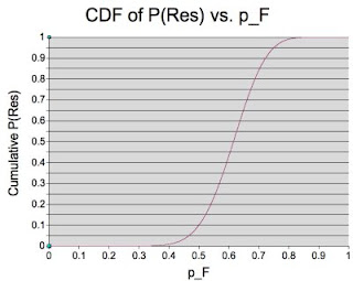

You can see that the peak of the PDF (I won't go into the terminology here, it's getting long) is indeed around 0.62 (0.6207, to be precise). But we're interested in a confidence range, for which we read off of the CDF the pF values for P at various levels. For instance, we're 95% certain that pF lies between the 0.025 level and the 0.975 level - i.e. between 0.4385 and 0.7734. We're 50% sure that it lies between the 0.25 and 0.75 levels - so between 0.5550 and 0.6734.
How does this help us? Well, it narrows down pF substantially - remember, we didn't have a clue what it was before. Now we can say with some certainty where it isn't - it's unlikely to be more than 0.7734 or less than 0.4385, eliminating almost two-thirds of the possible values at a stroke. It's as likely as not to be in the range [0.5550, 0.6734]. Can we translate this into a match probability for the next game? Of course. Again, it's a number-crunching exercise, but we get the following for our key values of pF:
..pF.. P(Set) P(2-0) P(2-1) P(Win)
0.4385 0.3307 0.1093 0.1464 0.2557
0.5550 0.6522 0.4253 0.2959 0.7217
0.6207 0.8075 0.6250 0.2510 0.8760
0.6734 0.8977 0.8058 0.1649 0.9707
0.7734 0.9825 0.9653 0.0338 0.9991
This tells us: the most likely probability of Federer beating Agassi in two sets is 87.6% (1.14), that it's as likely as not to be between 72.17% (1.39) and 97.07% (1.03), and 95% certain to be between 25.57 (3.91) and 0.9991 (1.001). In the event, the best available odds were 1.35 with Expekt - and depending on how much confidence-in-value we wanted, we would take those and reap the benefit of Federer's 6-3, 6-1 demolition job.
This system is, I have to stress, very basic and currently only works if the two players met in the recent past. In the next instalment, I might have a shot at a link function so we can rate players who haven't met recently - but have played a common opponent.
* easy to spell; difficult to stop spelling
Saturday, February 3, 2007
The Reverend Bayes and tennis probability
The Reverend Thomas Bayes was pretty much your archetypal dour, 18th century English Nonconformist minister. Except that he was a probability whizz, and gave us a law which has annoyed amateur statisticians for the better part of three centuries. It goes something like this: the probability of one thing happening given that another happens, is the probability of both happening divided by the probability of the other thing: P(A|B) = P(A & B)/P(B)
A typical example would be "Given that my girlfriend has two cats, at least one of which is female, what is the probability of her having two girl cats?" The probability of two cats both being female is (in our idealised world) one in four, or 25%. The probability of at least one female cat in two is 3/4 or 75% (FF, FM, MF all include a girl, MM doesn't). So the probability of a second girl given a first girl is (25%)/(75%) or 1/3 (33.33%) - higher than the 1/4 given no information.
It is natural that Bayes's Law should remind me of tennis, since I have spent a lot of time looking at both twisting my head from one side to the other. How can we use previous results to determine unknown probabilities? And how well do we know them?
We will need to broach the difficult subject of probability distributions. The easiest way (for me at least) to visualise a probability distribution is as a graph. The graph outlines a region of unit area* - the x axis is an outcome, often a continuum from 0 to 1 but not forcibly; the y axis is a mystical variable called probability density. You drop a pin onto the graph so that the point is equally likely to land anywhere in the region, and read off the value on the x-axis. You can see that the peaks in the graph correspond to more likely outcomes.

Let's look first at the PDF of the sum of three rolled dice. It peaks in the middle, around 10 and 11 - meaning that you're much more likely to roll 11 than 3. This makes sense - you have many more ways to roll 11 (27, I think) than to roll 3 (just one).
Some important distributions include the uniform distribution, which is a level straight line (all outcomes equally likely) and the normal distribution, which is a bell curve - outcomes near the mean are much likelier than ones far away.
What we're going to try in the next article is create a very simple tennis model and find how our knowledge about one game affects our knowledge of the next. Our strategy is going to be as follows.
We start with a uniform prior distribution of p, a variable that describes how likely one of the players is to win a single game. We then take each possible value of p (from 0 to 1) and see what the probability of the result of a known game would be, given that value of p. Out of that we get a likelihood graph showing what values of p are more likely than others - which can be converted into a PDF if we multiply by a constant. Given the PDF, we can determine confidence limits for our value of p - we want to be, say, 75% sure it's no lower than a given value so we can evaluate the odds on offer for the next game.
* at least for continuous PDFs. For discrete ones, the sum of the probabilities is one, which amounts to the same thing in the limit.
[This article and the next were originally one article. But I realised afterwards that I'd lost the thread somewhere and needed to explain things a bit better.]
Friday, February 2, 2007
More from the postbag and an experiment
Guess who?
Not a maths fight, just a genuine puzzlement, as (as i said) your recommendation of the double/triple/whatever flies in the face of accepted gambling wisdom. Obviously that doesn't mean they must be correct, but did mean I was intrigued anyway, the point I was trying to make was not about value - the double clearly offers more (that did blow my mind, but I accept it :)) but that, it seemed, over time the singles staker would grow his bankroll by more (which has to be good, yes?), and also that the double is actually a hidden bit of poor bankroll management, as the amount you'll be effectively whacking on the second outcome is (usually) too much in relation to your bankroll. I don't know if those two considerations are important or not.
I probably owe Splittter an apology, in which case sorry. On reflection, I think he is right - that even though the value offered by the double is better, it's a worse bet for your bankroll than the two singles.
How can that be so? Isn't a better-value bet necessarily better than a worse one? It would seem not - it's also necessary to factor in the probability. Which leads, of course, to the question of what constitutes the best bet in a a situation - would you rather have 1% value at 1.5 or 10% at 15? As Splittter's original maths showed (you wouldn't know it, because I didn't show it), the key is not value per se, but expectation.
For a given market, the fractional Kelly stake k is (p - (1-p)/(o-1)). If you win - which you'll do p% of the time - you pick up (p(o-1) - (1-p) = (po - 1). If you lose, as you do (1-p)% of the time, you drop your stake. Your expectation is the total of (the probabilities times the outcomes): p(po-1) - (1-p)(p - (1-p)/(o-1)). If you want to do the algebra, that comes out to be E = k(po-1).
The larger this is, the better the bet. Of the two examples above:
1) p = 0.6733, o = 1.50 => v = po-1 = 0.01*. k = 0.02, E = 0.0002.
2) p = 0.0733, o = 15.00 => v = po-1 = 0.10. k = 0.0071, E = 0.0007.
So the outsider - in this case - is a better bet. Returning to the bets in the last example (two singles with p = 0.37 and p=0.35, both with odds of 3.00, versus a double of p = 0.1295 and o = 9.00)
3) p = 0.37, o = 3.00 -> v = 0.11. k = 0.055, E = 0.0061 (much better than 2) above)
4) p = 0.35, o = 3.00 -> v = 0.05. k = 0.025, E = 0.0013
5) p = 0.1295, o = 9.00 -> v = 0.166. k = 0.021, E = 0.0034.
What does all of this imply? In general, if you have two different bets offering the same value, the one with the shorter odds (i.e., the more probable of the two) gives the higher expectation. The key equation is E=k(po-1): the higher the value of E, the larger your expected return.
Next time I'll hopefully generate some non-postbag-related material, unless Splittter provides more thought-provoking analysis and argument. I may get moving on probability estimation techniques. But that's hard...
* po-1 is, of course, our definition of value. Greater than 0, we're looking at a value bet.
Thursday, February 1, 2007
From the postbag: Doubles
Of course, Splittter is the only one writing to me at the moment, which makes me feel a bit like Willie Thorne in the Fantasy Football League sketches. Anyway, here is his wisdom:
Your post on doubles has been bugging me since I read it basically because the accepted gambling wisdom is simply "don't do doubles", full stop, no exceptions... yet your maths looked correct.
I had a sneaking suspicion that it had to do with your bet size relative to your bankroll, and that hidden in the double is the fact that you're essentially sticking an amount larger than your actual stake on the 'second' outcome.
So, to test that theory I imagined the following:
There are two bets for which you'll get 3.00: event 1 you reckon will come in 37%, event 2 35%, both clear value bets.
He goes on to analyse the situation in excruciating detail. As I refuse to be out-mathsed by anyone, let alone Splittter, I'll do the same but more clearly - and reach a slightly different conclusion. His experiment suggests Kelly staking.
With Kelly staking, you would place a fraction k = p - (1-p)/(o-1) of your bankroll on each bet. Your expected return is p(kB(o-1)) - (1-p)(kB) = Bk(po-1)
Betting singles, your Kelly stake on the first game is 5.5% of bankroll; on the second, 2.5%. The outcomes are as follows:
Win-win: (12.95%) +16.50%
Win-lose: (24.05%) + 8.23%
Lose-win: (22.05%) - 0.78%
Lose-lose: (40.95%) - 7.86%
The weighted average of these - trust me - is 0.73%.
By contrast, if you bet the double, your Kelly stake is 2.07% of bankroll, and your outcomes are:
Win-win: (12.95%) +16.5%
Any other: (87.05%) - 2.1%
So, on average, you come out 0.34% ahead. So far, so good for the singles. However, let's examine the bets in terms of risk vs. reward:
Expected risk for two singles: 6.99%
Expected return: 0.73%
Value for singles: 10.44%
Risk for double: 2.07%
Expected return: 0.34%
Value for double: 16.42%
You might argue that we're not comparing apples for apples - that if we're betting singles, we're forced to make the second bet even if the first fails. However, if we don't make the second bet, we do even worse - as you'd expect, failing to make a value bet lowers your expected return (in this case, to 0.66%). The risk in that case is fixed at 5.5%, making the value 12.00% even.
How about the order of the bets? In fact, it doesn't make a difference to the expected return. It does make a difference to your expected risk, though, which drops to 6.26%. That makes the value 11.66% - still lower than the double. Without the second bet if the first loses, the expected return falls to 0.34%, with a risk of 2.5%, making the value 13.59%.
My correspondent challenges me to prove things in general. I scoff, mainly because I ought to do some work. I may leave that for a later post.
All of which seems to show that a double on two value bets gives better value than two singles. The singles give a higher expected value, but at the cost of an increase in risk which reduces the value below the double's.
Tuesday, January 30, 2007
From the postbag: Arbitrage
Splittter writes to say:
Worth saying that, although the arbitrage is seductive as it guarantees profit on each market, to the mathematically inclined gambler it's still only worth doing if all bets involved are value in their own right. Basically because if they aren't, although you'll win every time, over time you'll win less than if you just backed the value ones. I'll leave you to 'do the math' though :)
Alarmingly, my poker-playing friend is quite right. Allow me to thank him for making the first post. Let's say there are two arbitrage situations, one where both bets are value, and one where only one is.
Situation one:
Heads 2.10
Tails 2.10
Total implied probability: 95.23%
The arbitrageur backs both at the same stake, and pulls down 10% of it whatever happens. The value bettor does the same thing, with the same result. Bully for both.
Now let's look at a situation where only one is value:
Heads: 2.25
Tails: 1.95
Total implied probability: 95.72%
The arbitrageur puts GBP1.95 on heads and GBP2.25 on tails, to win GBP4.38 less GBP4.20 = GBP0.18 whoever wins. Over 100 bets, he wins GBP18. The value bettor places GBP4.20 on heads every time. Over 100 bets, he wins GBP9.45 50 times (GBP472.50), minus GBP420 staked - a profit of GBP52.50, almost treble the arbitrageur's return.
The cost of this expected extra profit is volatility. Five per cent of the time, 40 or fewer heads will show up in 100 throws. In the case of 40 heads, he would win only GBP378, less GBP420, a loss of GBP42. How terrible. On the other hand, 5% of the time, there would be 60 or more heads, leaving him with a much increased bankroll- GBP567 - GBP420 = GBP147 profit, more than eight times as much.
Over a much longer time frame, the value bettor would be statistically certain* to make more money.
* that is, over a long enough time frame, you can make it as unlikely as you like that the arbitrageur would win more.
Sunday, January 28, 2007
Kelly staking
Mathematician John Kelly came up with a system for staking which maximises your expected return over the long term. This is going to be a load of maths, so look away now if you're not interested.
Assuming you bet a proportion k of your bankroll each time at odds o, after you win W and lose L bets, you have B' = B [(1 + k(o-1))W (1 - k)L]. We want to find the maximum of this, so we take the derivative and set it to 0:
dB'/dk = W(o-1)(1-k) - L(1 + k(o-1)) = 0.
Or, W(o-1)(1-k) = L(1 + k(o-1)). Since over the long term, W/L -> p/(1-p) (see earlier post on the Law of Large Numbers), we can substitute in to get:
p(o-1)(1-k) = (1-p)(1 + k(o-1)). A little algebra then gives us:
k = p - (p-1)/(o-1), the Kelly Staking formula.
That means, if you assess the probability of the outcome to be 50% and the odds are 2.10, you should stake 0.5 - 0.5 / (1.1) ~ 0.5 - 0.45 = 0.05: a twentieth of your balance.
That's a big gamble. After losing a few consecutive bets, your bankroll of GBP1000 would have dwindled like this:
1. Bankroll: 1000.00 Bet: 50.00
2. Bankroll: 950.00 Bet: 47.50
3. Bankroll: 902.50 Bet: 45.13
4. Bankroll: 857.37 Bet: 40.72
5. Bankroll: 816.65
In four bets, you've lost nearly a fifth of your bankroll! On the other hand, if you'd won, you'd be laughing:
1. Bankroll: 1000.00 Bet 50.00
2. Bankroll: 1055.00 Bet 52.75
3. Bankroll: 1103.03 Bet 55.65
4. Bankroll: 1174.24 Bet 58.71
5. Bankroll: 1238.82
And you're up almost 24%. Kelly staking is a wild ride. As long as your value calculations are right, you'll end up way ahead in the long run*. Occasionally you'll lag at the wrong end of the binomial distribution and look like you're way behind.
Some gamblers choose to use a slightly less volatile system called fractional Kelly, in which they split their bankroll into (say) five separate bankrolls and use only one for Kelly calculations. That dampens the volatility a bit, but does make for smaller gains when you're winning.
So long as your value estimation is correct and the law of large numbers takes hold quickly enough - and you can stand the wild fluctuations in your bankroll - Kelly staking is the most profitable system known to mathematics. Use it wisely.
* In the above situation, you'd need about 1800 bets to be 95% sure of breaking even or better.
Exotic bets
For some people, singles - betting on one selection in one event - simply aren't exciting enough, and they need to bet on several selections in several events.
The simplest multiple is the double. The proceeds of winning one bet (a stake of s at odds of d1) are reinvested as your stake in the other (at d2), so you win (s.d1.d2 - s) if both win. A treble is the same with three selections; an accumulator is the same with more.
Another common multiple is the forecast in racing. You predict the first and second place horses/dogs/etc (in order, for a straight forecast, in either order for a reverse forecast which costs twice as much for the same payout*. The winnings are calculated by a Secret Formula known only to the bookies. Exacta and trifecta bets are the same kind of thing, but with three horses.
Now comes the fun bit - exotic bets. The first of these is the patent: three singles, three doubles and a treble on the same three selections, all with the same stake. It thus costs 7 stakes. If all of the selections are at 1.83, you would need to win two to break even (3.66 from the singles, 3.34 from the doubles, minus 7 staked). You need odds of about 7.00 on each to break even with a single win, and three wins will make a profit at any stake at all.
A trixie is similar, but without the singles - so it's four bets: three doubles and a treble. This kind of bet requires at least two of your selections to win to get any kind of payout. At 2.00 each, if two of your selections win, you break even. Three winners, as before, bring you a profit at any odds.
A yankee consists of four selections and every combination of doubles (6), trebles (4) and a 4-way accumulator, making 11 bets altogether. Odds of 3.33 on each selection are enough to break even with two wins, whereas 1.56 would do the trick for three wins.
A lucky 15 adds four single bets to the yankee. At odds of 15.00 each selection, a single winner will break even. Odds of 3.00 will break even with two winners, while 1.52 will guarantee a profit if three of them win.
There are many other types, including the Super Yankee (or Canadian), involving five selections (all combinations except singles - 26 bets). A Heinz is the same thing with six selections (57 bets - hence the name), a Super Heinz the same with seven (120 bets) and a Goliath does the same with eight (247 bets). Lucky 31 and Lucky 63 are the same as Lucky 15 but with five and six selections respectively.
There are two main reasons that exotic bets are interesting. Firstly, for the average punter, there's the chance of a huge payout. If your four singles came in at 2.00, you'd win 8 stakes minus the four you placed. If you'd had a Super 15, you'd have won 80 stakes, minus the 15 you put in.
Secondly, and this is critical for us, they multiply value. This is best explained with a double, or else it gets really complicated. Let's say you have two selections you believe are worth 1.80, but the bookmaker has them available to back at 2.00. On their own, each would give a value of 11% - a nice markup. If you backed them in a double, the true odds of both winning would be 1.80 * 1.80, or 3.24. According to the bookie, the odds of the double are 4.00, giving you a value of 23%, more than double.
Unfortunately, the best odds are usually to be found at betfair, whose structure doesn't lend itself to simultaneous multiples. However, if you're prepared to do a bit of maths, you can figure out equivalent stakes for consecutive events - with the double example above, after the first selection won, you would place the entire winnings on the second selection. I'll see if I can knock up some code to determine optimal staking plans... at some point in the future.
* because it's really two straight forecast bets.
Saturday, January 27, 2007
Arbitrage
Um... this is a break from our regularly scheduled programming. We'll look at doubles and accumulators next time. Right now I wrote an article on Helium about arbitrage which I thought I should reproduce here.
Arbitrage is the practice of making two or more financial transactions in such a way as to tie in a guaranteed profit. An example in the stock market world would be to buy a share at one price and simultaneously sell it for a higher price.
In gambling terms, an arbitrageur backs all of the possible outcomes in an event in such a way that any outcome results in a profit. An example would be to back one tennis player at 2.10 with one bookmaker and his opponent at 2.10 with another (staking GBP1 on both). Whichever player won, you would win 2.10 less your stakes, making a guaranteed profit of 10p.
In general, if you are to back one player at decimal odds of d1 and another at d2, you can arbitrage only if 1/d1 + 1/d2 < 1 (in the above case, the sum is about 0.95); to guarantee the same profit in either case, you will need to place stakes in the ratio (s1/s2) = (d2/d1) (i.e., so your stakes multiplied by the odds are the same). This is intuitive - you need to put more on the favourite than on the underdog to get the same return. Your profit will be s1.d1 - (s1 + s2).
Asian Handicaps
OK, THIS time we'll talk a little bit about a specific type of sports betting. Asian Handicap betting is one of the most popular forms among serious soccer* gamblers, perhaps because the over-round is generally quite low**. On betfair, the commission is just 1%, the lowest it offers.
The original idea of the Asian Handicap was to get rid of the possibility of a draw. One of the teams would be given a head start of half a goal, so that a draw would be counted as a win for that team so far as the bet was concerned. If the teams were mismatched, maybe a goal and a half or more could be used as a handicap.
However, half goal head-starts are not the only possible way to eliminate to draw. Another way is to simply ignore it - in a zero-handicap game, if there's a draw you get your money back. Again, handicaps needn't be restricted to zero: one or two-goal handicaps are fairly common. If you backed a team with a two-goal handicap and they lost 1-0, you'd win your bet; if they lost 3-1, you'd get your money back. Only if they lost by three or more goals would you lose.
But not even that was enough for some people. Instead, quarter-goal handicaps were introduced. Now, obviously a quarter-goal handicap, taken literally, is just the same as a half-goal. But that's not what it means. Instead, a quarter-goal handicap comprises a pair of bets with the same stake, one at the handicap above and one at the handicap below. For instance, if you backed a team with a head start of 1/4, you would be effectively backing them with half your money at a handicap of 0, and half at a handicap of 1/2. If the team wins, you win both bets; if it's a draw, you win one bet and get your stake returned from the other; and if they lose... you lose too.
The next article will explore the mystical world of exotic bets, beginning with doubles and heading on to other types of accumulator.
* I apologise to anyone who is offended at me failing to use the word 'football'. I prefer to use 'soccer' and 'American football' to avoid any confusion.
** The over-round, or vigorish, is one minus the total of the implied probabilities for each selection. For instance, if Player 1 is available at odds of 2.00 and Player 2 at 1.80, the total probability is 0.50 + 0.44 = 0.94, or a 6% over-round.
Friday, January 26, 2007
ELO, Élö, it's good to be back
So far, I haven't said anything at all about sports or rating systems. The sports thing, well, that's only going to change tangentially. The thrust of this piece is going to describe one of the best-known rating systems, the Élö system. I'm going to get tired of the accents, which may not show up on all systems, so I'll revert to calling it Elo like everyone else.
Elo is primarily used for chess. The basic premise is to compare how well a player did over a given time frame - say the number of games he* won in a month - with how well he ought to have done, given his ranking and his opponents'. At the end of the time period, his rating is adjusted to take those games into account.
That description leaves at least two questions: how do we know how well he ought to have done? and, how do we adjust the rating afterwards?
How well the player ought to have done depends on who he's played - if he's played ten games against Deep Blue, he might be expected to win one, if he's really good. Against my girlfriend's cat Darwin? Probably seven, if Darwin's on form. In fact, the number of games he's expected to win is the sum of the probabilities of each individual game**.
All well and good. But how do we figure out the probabilities of each game, given the ratings? This, unavoidably, is going to require some maths. If you have a rating of, say, 1700, and Darwin (who's only just started playing chess) is ranked at 1500, you have a rating difference (D) of +200. From Darwin's point of view, it's -200. The probability of you beating him is 1/(1 + 10(-0.025 D))***. In this case, that's 1/(1 + 10-0.5), or 1/(1 + 0.32), about 0.76. For Darwin, if you'd like to do the sums, it's 1/(1 + 3.16), or 0.24. Note that the probabilities add up to one, as they ought to****. Over ten games, you'd expect to win 7.60, while Darwin makes do with 2.4. (Incidentally, he plays worse if you throw a ball for him to chase.)
So, let's say you played ten games against Deep Blue - we'll say it has an Elo rating of 2800 - (D = -1100 for you) your probability for each game is very small (0.18% - about one in 550). In ten games, you'd expect to win about 0.02. Let's say you did well against Darwin and picked him off eight times, and Deep Blue creamed you, as is its way. You won eight games (W=8), and your expected number of wins was E=7.62 - you did better than expected by 0.38 wins. Very good.
The last step of the process is to adjust your rating. A certain weighting (K) is given to your recent results - in chess, it's usually about K=12, but in later articles I'll hopefully determine what the best values for tennis are. In this case, your rating goes up by K(W-E), or 4.62 points. Your new rating would be 1705 (rounded off).
* or she. Take that as read pretty much everywhere in this blog.
** For the mathematicians: The expected number of wins is sum(p_i) +/- sqrt(sum(p_i . (1 - p_i))).
*** The 0.025 is arbitrary, but the only difference it makes (so far as I can see) is to the spacing of rankings.
**** ... so long as we exclude the draw as a possible result. Which we do, for simplicity's sake.
Thursday, January 25, 2007
The Gambler's Fallacy and the Law of Large Numbers
In its simplest form, the gambler's fallacy is to believe that, just because something hasn't happened for a while, it's due to happen soon. The usual example is a coin that comes up heads ten times in a row. The fallacious gambler thinks it has to come up tails soon - "the law of averages says it must!" But of course it needn't. The chances of the next toss being a tail remain 50-50, as they ever were.
There are occasions in which the gambler's reasoning might not be fallacious - for instance, if you were drawing cards from a pack without shuffling, each non-ace that was drawn would increase the chances of the next card being an ace - but in almost all gambling scenarios (at least in the casino and possibly excluding blackjack), there is no memory involved.
It's possible that the fallacious gambler is misremembering the Law of Large Numbers. This is a much misunderstood mathematical theorem - I once spent an entertaining breakfast arguing with a friend about this, much to the bemusement of everyone else in the backwater Wyoming diner. The Law says that, if you look at a random event for enough trials, the number of successes divided by the number of trials will get as close as you like to the probability. If you toss a million coins, you should end up with an observed probability of almost exactly 0.50. Unfortunately, that doesn't quite mean that you can put the bank on there being exactly 500,000 heads, though. In fact, the Law of Large Numbers even says how far away you can expect to be - in this case, on average you'll be within 500* tosses of that. I just ran a quick test, emptying my piggybank and tossing 1,000,000 coins a hundred times over**. I found:
So the experiment conforms pretty much exactly with what the Law predicts.
* in general, the expected number of successes, each with probability p in N trials, is pN +/- sqrt(Np(p-1)). The square root is a standard deviation; 68% of the time, the answer will lie within one SD of the mean (pN); about 95% of the time, it'll be within two.
** My piggybank is entirely virtual. Code and results are available on request; if there's enough demand I might make a little javascript to demonstrate.
There are occasions in which the gambler's reasoning might not be fallacious - for instance, if you were drawing cards from a pack without shuffling, each non-ace that was drawn would increase the chances of the next card being an ace - but in almost all gambling scenarios (at least in the casino and possibly excluding blackjack), there is no memory involved.
It's possible that the fallacious gambler is misremembering the Law of Large Numbers. This is a much misunderstood mathematical theorem - I once spent an entertaining breakfast arguing with a friend about this, much to the bemusement of everyone else in the backwater Wyoming diner. The Law says that, if you look at a random event for enough trials, the number of successes divided by the number of trials will get as close as you like to the probability. If you toss a million coins, you should end up with an observed probability of almost exactly 0.50. Unfortunately, that doesn't quite mean that you can put the bank on there being exactly 500,000 heads, though. In fact, the Law of Large Numbers even says how far away you can expect to be - in this case, on average you'll be within 500* tosses of that. I just ran a quick test, emptying my piggybank and tossing 1,000,000 coins a hundred times over**. I found:
- the average set of tosses contained 499,978 heads
- the standard deviation was about 460 - pretty close to what the Law predicts.
- 97% of the observations were within 1000 of the real mean
- 71% were within 500.
- None were exactly 500,000 (or even within 10).
So the experiment conforms pretty much exactly with what the Law predicts.
* in general, the expected number of successes, each with probability p in N trials, is pN +/- sqrt(Np(p-1)). The square root is a standard deviation; 68% of the time, the answer will lie within one SD of the mean (pN); about 95% of the time, it'll be within two.
** My piggybank is entirely virtual. Code and results are available on request; if there's enough demand I might make a little javascript to demonstrate.
The Search for Value
Almost any serious article about gambling will mention "value" at some point. Not many of them explain neatly what value is. They will generally give a few examples, assume you've got the point, and move on. So here, once and for all, is the definition of value: the value of the bet is the "real" probability of the result happening divided by the implied probability of the bookmaker's odds. If this number is greater than one, the bet constitutes value.
That seems simple enough. The implied probability might look a bit tricky, but it's not too bad. In decimal odds, the implied probability is simply one divided by the odds - so a team available at 2.00 to win have an implied probability of 0.50, or 50%. If the odds were 1.5, the implied probability would be two-thirds, or about 67%. Odds of 10.00 represent a 10% chance.
All well and good, if you're using decimal odds. What if you prefer the old-fashioned, 100-to-30 style favoured by men in cloth caps making odd gestures? Well, you're going to need to do a little more maths, I'm afraid. Odds in the style x-to-y against simply mean that the bookies imply the selection will lose x races for every y they win. X-to-y on is the other way around - they'll win x for every y they lose. Evens, or 1/1, means wins and losses are (implicitly) equally probable, 2/1 on* represents an implied probability of 2/3, and 9/1 against corresponds to a one in ten chance.
To convert fractional odds like these into implied probabilities, you take the number on the right (left if it's in the style of 2/1 on) and divide it by the sum of the two numbers - so it's the number of races you'd expect to win divided by the total number of races. You can easily see that 9/1 corresponds to 1/10 = 10%. (If you divide one by that, you get the decimal odds, 10.00.)
So much for the maths involved in working out implied probability. There are two burning questions that I can see I haven't answered. One, how do you compute the probability of winning? And two, why is value important? The first is one of the main things The Martingale will be looking into. The short answer is I don't know, but I hope to find out. I can answer the second, though:
A value bet is one where, if you repeated it often enough, you would win more money from winners than you lost from losing. For instance, if a horse was at 10.00 and you figured it had a one-in-eight chance of winning**, over a hundred races you'd expect it to win about 12 or 13 times. Each time, you'd be returned $10 for a $1 stake. So you'd get, let's say $125 back from the bookie after giving him only $100 - a profit of $25. The value (minus one) is the return (here, 0.25 or 25%) you'd expect on your money over the long term if you made bets at that value.
In the next article, I'd better talk about the gambler's fallacy and the law of large numbers.
* This also gets written as 1/2, in which case the first definition is correct - the selection loses one race for every two it wins.
** (1/8) / (1/10) = 10/8 = 1.25, so this is value.
Wednesday, January 24, 2007
The Martingale
You're in the casino and place a $1 bet on red. It doesn't come up, so you place a $2 bet on red, so that if you win you pick up $4 - everything you've staked so far, plus a dollar. It misses again, so you bet $4 - the $8 you'll surely win THIS time covers all you've staked - $1 + $2 + $4 = $7, plus a dollar to win. Red's bound to come up eventually, so eventually you'll make your dollar. It's a foolproof system! It's called the Martingale, and - unfortunately - it doesn't work very well.
The word martingale derives from the town on Martigue in Provence, southern France. In Martigue, where trousers were traditionally worn fastened at the back. "A la martingale" soon came to mean 'in a ridiculous fashion' and is applied in exactly that sense to the system above.
The problem with the Martingale is that your bet size gets very big very quickly - as you can see below.
Bet number: Stake size
1: $1
2: $2
3: $4
4: $8
5: $16
6: $32
7: $64
8: $128
9: $256
10: $512
After losing ten bets in a row (which will happen a little fewer than once in a thousand times*), you'll be looking to gamble over $1000 dollars to win just one in return - and the odds you're getting are still a little worse than evens. Yes, you're bound to win your dollar in the end - as long as you have an infinite bankroll. Eventually, you will simply reach a point where you don't have enough to carry on playing, and you have to stomach a devastating loss.
* Actually, in a casino the odds are slightly worse than this because of the house edge. In an American casino with two zeroes, the probability of red is about 0.47 rather than the 50% implied by the odds. That makes the probability of ten losing red bets in a row about one in 610.
Welcome
My name is Colin and I'll be your guide to all kinds of gambling and probability-related maths in this blog. I'm happy to field questions and try to put right any errors you find. I ought to emphasise the DISCLAIMER:
The Martingale comes with absolutely no warranty of any description. You can use information contained herein any way you like (although if you republish it anywhere, you must include the disclaimer in full as well as a link to the original article), but it's not my fault if you lose all your money. Gambling may not be legal depending on how old you are and where you are. If you get busted, that's not my fault either.
You might well ask - why are you sitting here writing a blog instead of ripping Vegas to shreds, if you know so much about gambling? It's a fair question. My interest is more in sports betting than casino gaming, and I'm currently based in the US where such things are generally illegal - or at best, awfully shady. I'm also the kind of mathematician who's much more interested in solving complex probability puzzles than making much money using them. Which is why this is all free and accessible to everyone.
It's called The Martingale after a staking system that doesn't work, described in the following post. The url is martegal.blogspot.com because martingale was taken, and martegal is the Portuguese word from which Martingale was derived.
Subscribe to:
Posts (Atom)